Saturday, May 3, 2025

Years ago, I sat down with Charlie Munger for a private lunch in Omaha; it was a priceless experience, and we’ll never forget it. It was a special day with a legend, all laid out in our latest book, When Markets Speak.

Today, our trusted Bear Traps Report associate, Chris Davis, is there.

NY Times Best Selling Author, Larry McDonald

Live From Omaha, Nebraska.

Today, HVP’s Marino Patrk and Christopher Davis attended the Berkshire-Hathaway Annual Meeting in Omaha, NE, and have been in town since Thursday. They attended conferences held by Gabelli Asset Management and Columbia Business School’s Heilbrunn Center for Graham & Dodd Investing and visited the over 20,000-square-foot exhibition of products and services that bring the sprawling conglomerate to life.

Throughout the meeting, Mr. Buffett returned to the phrase “turn every page” as an investor on the hunt for ideas and knowledge. It was not until the very last page, however, that Mr. Buffett made his big announcement—that he would advise the Board of Directors to have Mr. Greg Abel succeed him as CEO at the conclusion of this year.

At nearly 95 years of age, Buffett’s record as the greatest investor of all time stands firm. His recall of both current events and those 60-70 years ago was incredibly strong throughout the over 4 hours of question and answer. Buffett’s commonsense approach to investing, policy, and living has been a timeless draw for shareholders from all over the world. It was the late Charlie Munger who let slip a few years ago in a meeting that “Greg would preserve the culture,” and in subsequent meetings, it became more and more apparent that the leadership transition had happened without fanfare and under our noses. Buffett’s comments today also affirmed his support of Abel in that he plans to keep every share he has in the business. He qualified that it was an economic decision, “because I think the prospects of Berkshire will be better under Greg’s management than mine.” A truly breathtaking statement from the man who turned a failing New England textile mill into a trillion-dollar business, hitting all-time highs in price with Friday’s close.

Berkshire-Hathaway is a cornerstone holding across all strategies and portfolios at Hudson Value Partners. Mr. Buffett’s 60 years of stewardship have been nothing short of exceptional. Like him, we have confidence in Mr. Abel and all of Berkshire’s managers to navigate the challenges and opportunities of the decades ahead with the same discipline, ingenuity, and integrity that have benefited Berkshire-Hathaway shareholders for 6 decades.

Below we will share the top 5 ideas that came up in our conversations as a firm, at conferences, and with investors from around the world from the past few days in Omaha:

Institutional investors can join our live chat on Bloomberg, a groundbreaking venue since 2010 – now with clients in 20+ countries; just email tatiana@thebeartrapsreport.com – Thank you.

Pick up our new best-selling book — “When Markets Speak“ – On Amazon today.  Below is a short but essential light on the book’s intelligence gathering.

The Legendary “W” Games

Over the last 250 years of American political gamesmanship, both parties have played year-end games into the arms of a new incoming administration. In early 2000, the incoming George Walker Bush team discovered that every keyboard in the White House and other administrative offices was missing the “W” key¹. The outgoing Clinton staff had removed all the “W” keys to annoy the new administration after an extremely contentious election. The damage was small, estimated at $15,000. But the bigger message here was that when the party that runs the White House changes, the outgoing administration will leave some proverbial “time bombs” for their successors.

While the damaged keyboards were more like a bad joke, what Biden is doing to Trump now is serious business. The outgoing administration has opened the spigots table max to get every penny out the door while they can under the existing budget. It’s almost like they are looting the Treasury before they leave town.

Biden is Opening the Floodgates with Spending
Spending for 2025 is expected to exceed $2Tr by the time Biden leaves DC on January 20^th. This is over 30% of the annual budget, and Trump will have to cut spending for the rest of the year to stay within the limits of the allocated budget. This could mean a notable slowdown in GDP growth in the first quarters of 2025.

Bonds have taken Notice
Ever since the Fed cut rates in September, U.S. 10-year bond yields are about 1% higher, and mortgage rates are following in lockstep. Hedge funds are selling short, betting on lower bond prices into colossal incoming bond sales from the U.S. Treasury. This is a highly unusual activity and has the fingerprints of the bond vigilantes everywhere; a revolt is in the works.

Lunatics – as Usual – on Capitol Hill 

Congress, in its usual fashion, has failed to agree on the next budget, so the government is currently operating under a “continuing resolution” (CR). This continuing resolution means the government is allowed to spend the same amount of money they spent last year, which is $6.75TR. The government’s fiscal year started on October 1^st, and Biden is on a run rate to spend almost $2TR by the end of December and a deficit that may exceed $800bl (+60% y/y). So, when Trump comes in on January 20th, he has three quarters left of the government’s fiscal year, but by then, Biden has spent more than 30% of the total allocated budget. This forces Trump to cut spending right off the bat. We estimate spending could drop by $500bl quarter over quarter, or 25% from Q4 to Q1. This is an estimate, and the timing of spending can change. But the fact is that Biden is emptying the coffers before Trump gets in. Every week, more money and weapons are sent to Ukraine, more subsidies are given to semiconductor makers to build plants in the US, and more government employees are hired.

US Yields Surge While Others Languish
Since September, US Yields have surged over 20% on Biden’s sugar high, while Canadian and German yields are down since then, Chinese yields have collapsed, and UK yields are only modestly above the September level.

Government Job Growth Twice the Rate of the Private Sector
Private sector job growth has lagged government job growth significantly in the last year as the government keeps hiring people.

Why is this so Bad?

We believe that this spending deluge by Biden on his way out is partially to blame for the surge in bond yields in Q4. Some may say it’s because of Trump and his promised tax cuts, but the Republican House majority is so slim that it’s unclear how much of a fiscal stimulus Trump is actually able to get through Congress. Also, the incoming Senate majority leader Thune (R, SD) has said he will only get one bill through reconciliation in FY 2025 and another one in FY2026. His priority is on immigration and energy legislation, so a fiscal spending bill might not come until late 2025 or early 2026 if anything. But if yields are being pushed up by all this spending in Q4, then what will happen if spending falls back in early 2025? And what will happen to GDP growth? A $500bl drop in government spending from Q4 to Q1 is the equivalent of 1.7ppt of growth. So, if Q4 nominal growth comes in at 5.7% annualized, this could drop to 4% in Q1 if government spending slows down accordingly.

Treasury’s Reliance on Short-Term Debt Exploded in Recent Years
Election Rigging? We are witnessing a Covid era like spending in 2024 without a pandemic. The Treasury Department has come to rely on short-term bills to fund the government. But with $36Tr of debt, the Treasury has to issue bills almost every day to keep funding the government and to refund maturing debt.

Interest Payments on the Federal Debt Load

2026: $2.1T?
2025: $1.5T?
2024: $910B
2023: $658B
2022: $475B
2021: $352B
2020: $224B

*CBO data, Bloomberg. The average weighted coupon on the U.S. debt load is about 2.7% vs. over 4.5% for 10-year U.S. Treasuries. As bonds mature, they get refinanced at much higher yields.

$10Tr of Debt Refinancing Next Year

In 2024 Treasury faced around $10Tr of maturing debt. To refinance this debt, it issued a whopping $26Tr of bills and bonds. More than 84% of that paper was short-term bills with a maturity of 6 months or less. Treasury keeps re-issuing bills with a maturity of 4 to 8 weeks or 3,4 to 6 months, which are the most popular maturities in a continuing, ever-increasing roll down of the debt, day after day, month after month.

Apple Long-Term Bonds and Interest Rates
ALERT – By issuing nearly a colossal load of extremely short-term bills, Janet Yellen succeeded in suppressing bond volatility in an election year and, in our view, strategically placing that bond market volatility into 2025 after the election. You can “why” see above, she wanted LESS long-term paper in circulation markets in the election year. Now, in 2025 – this paper has to be rolled over and termed out into longer-dated bonds. The USA is behaving like a financially trapped emerging market country. Living on the “front-end” of the yield curve is a VERY dangerous game.  The Apple AAPL 2.55% bonds due 2060 are trading down at 57 cents on the dollar. If long-term bond yields go to 6%, take a guess where this bond will trade. Near 47 cents on the dollar? Now think of the trillions of USD loans issued in 2017-2021 on bank balance (commercial real estate, mortgages, corporate debt outstanding). Losses are in the trillions of dollars with higher incoming interest rates. 

Interest Rates UP – Bond Prices DOWN
Never, ever forget that 6% today is equivalent to the destructive capacity of 10% twenty years ago. Interest rates up, mean bond prices down. A 1% move in interest rates higher today is an entirely different, far more lethal equation.

Incoming Stress Points

In 2025 the U.S. Treasury faces $9.6Tr of maturities in their so-called publicly held debt. In Q1 alone — the government faces $5.58Tr of maturities (bonds coming due, redemption), but 86% of those are short-term bills that the Treasury department rolls over into new 4-week, 8-week, 3,4, or 6-month bills, among others. As a result, almost daily bill auctions are coming to a theater near you, as the Treasury Department mindlessly keeps pushing new paper into the market to pay back the colossal amount of maturing debt.

Is There Any Reason to Buy Treasuries?

The new Treasury department under Scott Bessent may reduce bill issuance a bit and increase coupon paying issuance, just to alleviate some of the pressure on the bills market and extend the duration of outstanding US debt. Now that the big slush fund that bought all these bills, the so-called Reverse Repo Facility (RRP), is close to being depleted, it will be harder to sell all that short-term paper. In addition, Goldman Sachs expects that the Federal Reserve will stop the run-off of treasuries from its balance sheet by the end of January and begin buying treasuries again with the proceeds of the maturing MBS on its balance sheet. As such, the Fed becomes a modest buyer of treasuries next year, which allows the Treasury to increase coupon issuance without disrupting the long end.

One big bullish catalyst for treasuries would be a regulatory change to exempt treasuries from the Supplemental Leverage Ratio (SLR). It is unclear if and when this would be implemented, although Bessent was hinting at regulatory relief for banks to boost banks’ treasury holdings. Exempting treasuries allows banks to hold more Treasuries on their balance sheets without needing to hold additional capital against them, freeing up the capacity for banks to participate more actively in the Treasury market. Its unclear how much treasury demand that would create, but in 2021, when the temporary SLR exemption was reinstated after COVID, prime dealers reduced their Treasury holdings from $250bl to $125bl in 2 months. A change in the SLR ratio may come but is going to take months before the rules are changed. A phase-out of QT for treasuries would be a more immediate, albeit more modest, relief for the bond market. According to this timeline, the Fed will end up buying $100bl of treasuries in 2025, a big change from the $500bl of treasury sales in 2024.

¹https://www.latimes.com/archives/la-xpm-2002-jun-12-na-clinton12-story.html

The Fed has been Politicized

We have been very critical of Yellen’s term at the Treasury, but upon some further reflection, we think it’s really the case that Yellen’s only real issue was acting in the short-term interests of her boss and her party as opposed to thinking longer-term about how the government finances itself on a sustainable basis.

Her decision to fund the government with T-bills over duration securities and violate long-standing Treasury Department “norms” was incredibly short-sighted, but as someone who works for the President, ORDERS to follow.

Many have been super critical of her for these decisions because she should know what they would lead to and how really what she (and Powell together) has done is favor asset owners and the wealthy over everyone else in America, exacerbating wealth inequality to precarious levels in this country while still not bringing inflation back down to target. So ultimately, her decisions got her team knocked out of office anyway.

Looking forward, though, the issue is that there is no one in the government who is really thinking about and acting on behalf of the longer-term interests of the country when it comes to how much debt we are raising and how we are financing the government. The myopia about these decisions to get the existing political party in control through the next election is incredibly concerning.

The Fed has said this is not their lane; however, they are elected to 14-year terms and are supposed to be above politics. There are things they could have done to offset the politicization of the Treasury. They chose not to, they continue to protect asset holders and the Treasury market, decisions that really just make them become political as well. They could have better neutralized Treasury’s political decisions through more active QT, actually selling securities instead of just rolling them off, not adding to their duration holdings such that the weighted average maturity (WAM) of their positions is longer than Treasury’s own WAM. Powell’s Fed needs to be getting way more criticism than they are currently about these decisions which have made it harder to bring inflation down for the average American.

So if the Treasury is not going to think long term and the Fed is not going to either (the Fed actually is complicit because they don’t allow any real treasury market dysfunction to exist, which would be the way to deal with these long term issues by having the market / bond vigilantes do their thing), then who will? This is a problem, the bond market is starting to figure it out, term premiums are starting to normalize and the new administration will have to make some big decisions early on in their term.

Maybe @elonmusk and @DOGE can look into this as well. Someone has to!

With Robbert Van Batenburg, Craig Shapiro, and Larry McDonald.

Institutional investors can join our live chat on Bloomberg, a groundbreaking venue since 2010 – now with clients in 20+ countries, just email tatiana@thebeartrapsreport.com – Thank you.

BRICS+ Three-Day Summit at Kazan

A core thesis of our new book — “When Markets Speak“ is found in the hubris in Washington around the USD. A) sanctions abuse over 15+ years by the GOP and Democrats, and B) property confiscation (Russia) are the catalysts. What are the long-term side effects? Global public debt tripled since the mid-1970s to reach 92 percent of GDP (or just above $91 trillion) by end-2022. In recent years, as interest rates surged, global central banks are now collecting MUCH HIGHER coupons and interest. We believe – as stated in “When Markets Speak“ – that a significant part of this excess cash flow, central banks are putting / will place that overflow interest in gold and other hard assets — away from USD.

Planet Earth and the USD

In private transactions, per the IMF, although the United States only makes up a quarter of global GDP and just over 16 percent of world exports and imports, the U.S. dollar continues to be represented at a disproportionately higher rate in financial transactions. Approximately half of all cross-border loans, international debt securities, and trade invoices are denominated in U.S. dollars, while roughly 40 percent of SWIFT messages and 60 percent of global foreign exchange reserves are in dollars. Per the NY Fed, the percentage of foreign currency debt denominated in U.S. dollars has remained around 70 percent since 2010.

The Summit

Putin opened his remarks at the largest foreign policy event ever hosted by Russia by formally acknowledging the Kazan declaration which covers the following topics. 1) Ukraine should be resolved through diplomacy; 2) concerned about Gaza, the West Bank and Lebanon, Israel’s military offensive, the loss of civilian lives; 3) objects to sanctions; 4) expresses a need to reform the international financial system; 5) establishes a grain exchange and trading platform called the BRICS Grain Exchange which will eventually cover all agricultural produce; 6) seeks to develop the BRICS Interbank Cooperation Mechanism (ICM) which will focus on financing of local currencies and other financial practices; 7) affirms support for the IMF; 8) affirms support for the G20; 8) affirms the need to protect species of large cats.

Review of Putin’s Speech:

He stressed that business activity is shifting towards emerging markets. He pointed to the debt loads of developed countries and protectionism as destabilizing geopolitically and fragmentation of international trade which in turn causes inflation. He believes BRICS countries are more fiscally responsible. He believes the purchasing power of the BRICS is greater than that of the G7 and will grow. As a result, he believes BRICS should enhance coordination in technology, resources, trade, logistics finance, insurance and capital investment. A key focus is the sustainability of supply chains. He claims that fighting global warming is a means to suppress BRICS+ economically. He is for establishing a BRICS arbitration center to resolve internal disputes. He stressed that the establishment of a BRICS grain exchange will protect BRICS countries from external interference. He wants a full-fledged commodity exchange. He pushed for further cooperation in mineral exploration. According to him, the minerals market is hampered by trade barriers, which wants to see dropped within BRICS. He wants to see better transport connections between BRICS countries. Another significant goal of his is to cooperate on Artificial Intelligence.

Our Read:

This was Putin’s laundry list of everything he could think of that he wants. We didn’t know he liked big cats so much! In any case, there was a sense of “Together, we are bigger than Russia’s enemies” which, intriguingly, implies Russia cannot go it alone.

Review of Xi’s Speech:

After bemoaning the situation in Ukraine and Gaza, Xi shifted to greater cooperation in Artificial Intelligence among BRICS members. He pointed out China’s role in providing minerals for technologies that reduce carbon emissions. He believes legal governance for what he termed “the Global South” needs to be reformed. He wants further financial and economic coordination and towards that end lauded the New BRICS Development Bank. Overall, his remarks were much less specific than Putin’s.

Our read:

The only thing Xi wants is a financial system not dominated by the West, plus all the minerals he can lay his hands on, and he wants it in a legally binding way to China’s advantage.

Review of Sissi’s Speech:

He stressed Egypt’s desire for a multipolar world so that the developing world can be placed on a path of sustainable growth. He expressed pride that the first meeting of the New Development Bank was held in Egypt this past June.

Our read:

Basically, he will agree to anything if the other BRICS countries give Egypt more money.

Review of da Silva’s Speech:

He video-conferenced his speech from Brazil, saying that BRICS represent 36% of global GDP, and within BRICS territories is 76% of the manganese, graphite, and rare earths of the planet. He too stressed the importance of creating a financial system to reduce costs between BRICS members. He celebrated that the New Development bank is now 10 years old and is considering $100 billion worth of projects. He pointed out that he does not want to replace domestic money, however. Brazil will have the Presidency of BRICS for the year going forward.

Our read:

He wants the benefits of expanded BRICS powers without risk to Brazil’s sovereignty.

Review of Modi’s Speech:

BRICS accounts for 40% of the global population and 30% of the global economy. He is happy that the New Development Bank has current projects worth $35 billion. He wants the bank expanded. He wants more infrastructure projects. He is in favor of greater financial consolidation among BRICS members. Towards that end, he thinks the Unified Payment Interface developed by India and used between India and the UAE is working well and should be expanded throughout BRICS members.

Our read:

He wants more infrastructure in India and wants money for the projects to flow freely.

Review of Pezeshkian’s Speech:

The representative from Iran complained about the one-sidedness of Western hegemony and that the expansion of BRICS into BRICS+ is part of that solution. He wants the US dollar’s dominance to be reduced. He favors a BRICS currency basket. He believes the New Development Bank and the Reserve Fund should address the problems of payment imbalances and favors an integrated electronic platform to enhance trade between BRICS+ members.

Our read:

Iran’s membership in BRICS+ is a defensive move viz a viz the West.

Overall impression:

BRICS+ wants to reduce the influence the United States has on global trade and finance. The BRICS currency system is being avidly pursued, and Putin was actually given a BRICS currency bill at the summit, over which he beamed. We think that on the surface, the talk was about finance, currency and trade, but that under the surface it was about Russia, China, and Iran thinking militarily and the rest of the members thinking about how to make more money. As such the latter group seemed just a touch more cautious than the former. It is telling, too, that Xi said the least. He would like to hide his cards, but the reality is he wants China to dominate the world militarily and economically. Furthermore, the “Global South” is really about Africa and its mineral deposits. Finally, and not surprisingly, for all the talk of unity, each country seems to care about itself and its agendas most of all. We think that multipolarity will continue, but we doubt the US will become a non-entity. We maintain our view that after a meaningful decay (continued loss of market share), the US Dollar will still remain the dominant currency in world trade and finance and that a pruning back of that dominance to some small degree will actually give the Treasury and the Fed greater flexibility. The dollar will not be replaced. It will be given more room to maneuver.

Institutional investors can join our live chat on Bloomberg, a groundbreaking venue since 2010 – now with clients in 20+ countries, just email tatiana@thebeartrapsreport.com – Thank you.

A special thanks. Our latest book “When Markets Speak“ has been in the top #10 on Amazon over the last several weeks across most non-fiction, finance categories. We appreciate your support.

It’s that time again. In this blog, we will discuss the setup for the 2024 US elections, what the key states are to win for the candidates, and what the probabilities and polls tell us. We discuss specific stocks to play for a Trump or a Kamala win, and why the outcome of the Congressional elections is critical for your positioning in both equity styles, currencies, and fixed income. In sum, a sweep on either side, whereby the candidate also wins both chambers of Congress, would be bearish for bonds, as it means higher GDP growth and more spending. This would be bullish for cyclicals and small caps (IWM) and Emerging Markets (less tariff risk) in Trump’s case. In Kamala’s case, the market may get spooked by prospects of higher corporate taxes. Some income groups might sell stocks ahead of higher capital gains taxes as well. Equities could see a correction, which means defensives outperform.

*Special thanks to our long-time associates at ACG Analytics in Washinton, we highly recommend their fine team on the policy consulting side of the business.

Regional Banks, Pricing in De-Regulation
Our friend Stan Druckenmiller is NO Trump fan. He has NOT endorsed the former President, but he made an important point last week. When you look at a) the polls, b) the betting sites, and c) the Trump trades combined, they all are moving, quite sharply in the same direction over the last 12-14 days. Observe the Regional Banks – up +34% since mid-June vs. just +12% for the S&P 500. This sector is pricing in a significant De-regulatory regime.  As you can see above, this week the KRE pierced its upper Bollinger band, which doesn’t happen very often and is a sign of real FOMO, fear of missing out.

Regional Bank Strength, Lessons from the 2016 Election
Regional banks love deregulation, look at the – vertical – price action of Texas Capital Bank in 2016 around the Trump victory, and now look at TCBI’s daily relative strength, near the highest levels in a decade. 

Private Prisons
We host a conversation on the Bloomberg terminal with institutional investors. There are several portfolio managers we respect – all making the same point. “GEO ($15.20 Friday’s close) is up 100% from here in a Trump victory scenario. Our analyst says $45.” Trump has promised to be a “law and order” President. GEO equity is 30% off the Democratic National Convention lows. Markets are speaking here. 

*The GEO Group, Inc. operates private correctional facilities located mostly in the United States, and other countries. The GEO Group specializes in the ownership, leasing, and management of secure facilities, processing centers, and reentry facilities and the provision of community-based services. Its worldwide operations include some 110 maximum-, medium-, and minimum-security correctional, detention (including immigrant detention), with roughly 80,000 beds. It also conducts community supervision of offenders and pretrial defendants.

“A Trump/Vance/RNC victory would clearly be more favorable for sector revenues and investment potential–but take exception to viewpoints that a Harris/Walz/DNC outcome would be nothing short of “catastrophic.” Rather, we present a framework for an asymmetric risk/reward opportunity for the group (and GEO in particular) with potential upside returns (under Trump) far in excess of probable downside risk (Harris win). ” Jones Research.

“Larry, I can say two things with certainty, 1) I don’t like Trump and have NEVER voted for him, but 2) if the race was for a fact “tight”, GEO equity would NOT be moving higher 4 out of every five days this month.“ CIO LA.

A Divided Government, Implications?

Remember, a divided government means FAR FAR, we mean FAR LESS fiscal stimulus and in Trump’s case imminent trade frictions. In Q1 this year the CBO stated the projected annual deficit would be $1.6T, now we are close to $2T.  A large fiscal cliff would appear in a divided government. Over $1T of spending cuts could be forced onto the scene. The current debt ceiling EXPIRES in Q1 2025, buckle up. Over time this would be bullish for growth stocks, which tend to outperform when GDP growth is muted, and bearish for Chinese exporters. But initially, the shock of less government spending supporting the U.S. economy would likely crash the stock market.  For bonds, this is a preferred scenario because it means less room to increase spending. When yields go down due to a change in domestic conditions, the dollar tends to decline as well, so gridlock is dollar-bearish.

Trump vs Kamala

Trump’s odds surpassed Kamala’s odds late last week as polling numbers tighten, and the race comes down to Michigan.

Electoral College Map – No Tossup

The Presidential election is won in the Electoral College, and not via the popular vote. Any candidate that wins 270 or more Electoral College votes wins the election, and these votes are distributed among each of the 50 states based on the population of each state. This year, the road for both candidates to the White House seems to go through Michigan. The map here shows each state and how they will vote based on the current polling aggregate of that state. The only one that is still too close to call is Michigan, so the battle will always be in the swing states but this year primarily Michigan. Note that Trump visited Michigan last week and will be back in Michigan this weekend.

Trump and the Curve Steepener
We must listen when markets are speaking.  When Trump won the 2016 election, the spread in bond yield between the two-year and 10-year U.S. Treasury widened, or what we call “curve steepening” (see top left above). Now look at the last 3 months above, the curve is steepening again into the 2024 election. Everyone knows Trump wants to cut taxes with a $35T national debt, we believe this will frighten many global investors and push up long bond yields in the coming months if Trump wins. More treacherous, in recent years, U.S. Treasury Secretary Janet Yellen issued close to $4T of T-Bills. In our view, much of Uncle Sam’s borrowing is front-end loaded and MUST be termed out next year.

A Colossal Wall of Debt
From 2024-2026, close to $15.5T of U.S. debt is rolling over. In the 2024 election year Janet Yellen wanted stocks higher and markets as calm as possible. What did she do? The U.S. Treasury recklessly sold an absurd amount of T-Bills in recent years. Longer-dated bonds move FAR FAR, we mean FAR more in price than T-Bills maturing less than one year. By issuing a crazy amount of T-Bills, team Yellen was able to suck a lot of bond volatility out of the market in an election year. Anything to help Joe and Kamala. The next Treasury secretary must term out some of this debt and sell longer-dated bonds into the market. We believe this will create some HIGH drama in the first half of next year. As you can see above, the average weighted coupon on the U.S. debt load touched 2.3% this year. It’s now close to 2.6%, BUT a ton of debt is coming due and front-end rates are still very high.

The Curve — U.S. Treasuries

3-Month: 4.62%
6-Month: 4.43%
12-Month: 4.18%
2-Year: 3.94%
5-Year: 3.87%
10-Year: 4.08%
30-Year: 4.40%

*Bloomberg data, yields on U.S. Treasuries. As U.S. Treasuries mature, they will be re-sold to investors at MUCH higher bond yields. Interest on the U.S. debt load is already at $1.1T vs. $4.9T of tax receipts. HIGH ALERT — We are in a dangerous zone, interest payments as a % of tax receipts are approaching 24%. For most AAA-rated countries globally, this number is closer to 4-8%.

Gold and Silver – Reckless Deficts are the Driver
In recent client trade alerts, and well documented in our latest bestselling book – “When Markets Speak” – we have been pounding the table silver bulls. Protectionist policies coming out of both the Harris and Trump campaigns are a game changer – a whole new sustained inflation regime is upon us. It’s been more than 75 years since we had a U.S. election in which both candidates supported the aggressive use of tariffs. We have entered a whole new world. Likewise, Trump tax cuts and $2T annual deficits coming from Biden – Harris are driving capital into hard assets and Bitcoin. The 2010-2020 portfolio is history, you need a 1968-1981 portfolio construction, reach out to tatiana@thebeartrapsreport.com for more information.

**We have been long silver in our high-conviction portfolio for more than three years. We normally buy and sell 1/3 of the position to take advantage of volatility, but have always stayed long silver since 2020.

Early Innings
This chart measures the relationship between the SLV Silver ETF and its 200-day moving average. We can get a feel for the state of play, how much momentum is on the field today is the question. As you can see above, the SLV is only 21% above its 200-day moving average. Past bull markets for silver reached 75%, 65%, and 33%, we are still in the early innings. We believe both Harris and Trump are silver bullish, Neither has a plan for reducing the U.S. debt trajectory. Likewise, the Fed has likely softened the path forward for political reasons. They just cut rates 50bps while their own Atlanta fed GDP now data is up at 3.4%! Throw in a fresh China stimulus plan and $2T annual deficit in Washington, and the probability of another inflation surge is high. Bullish silver. 

Russell 2000, IWM and the 2016 Election
IWM shares ripped 54% higher in the months after the 2016 election. This week, the Russell 2000 reached 11% off its September 2024 lows vs. 8% for the S&P 500.

A Look at the Important States

To make things more complicated, Michigan is one of the few states whose ballot has all the candidates that are running in this election. This includes Chase Oliver (Libertarian), Randall Terry (U.S. Taxpayers), Jill Stein (Green), Robert F. Kennedy Jr. (dropped out but still on the ballot there), Joseph Kishore (Independent—Socialist Equality Party) and Cornell West. These candidates will draw votes away from the main candidates, and the question is by how much. Some say Hillary Clinton lost Michigan in 2016 because of Jill Stein.

Michigan Polls

Polling data in Michigan show a very close race, but Trump is ticking ahead of Kamala in recent polls.

Trump’s Advantage in the Electoral College

In the multicandidate polling, which includes Jill Stein (Green party), Kennedy (dropped out), Oliver (Libertarian) and Cornel West (Independent) Kamala leads Trump by about 2pct points. All these candidates will be on the ticket in key states such as Michigan, N. Carolina, Wisconsin, and Arizona. So the most important polls are those that include all candidates, in stead of polls that answer the question, “if left with the choice between Trump and Harris, who’d you vote for?”

2016 Election Polls

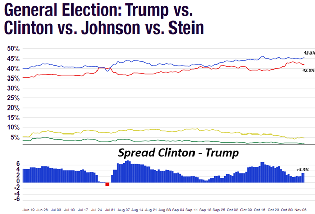In 2016 the final spread between Clinton and Trump was 3.3pct points. With about 136ml people voting, that 3.3pct points is 4.5ml voters, which is roughly by how much Clinton won the popular vote. It wasn’t enough for her to win the Electoral College, because most of those 4.5ml extra votes resided in New York State and California, which she has won regardless.

2020 Election Polls

In 2020 the final spread between Biden and Trump was 7.2pct points. With 158ml voters, that translated into a lead of 11.3ml votes. Biden won the popular vote by a margin of 7ml votes, and we account the difference to polling errors. The polls here are two-way because Democrats were effective in litigating Green Party candidate Jill Stein off the ticket in most states.

The point is that Bidens 7.2pct point lead in the polls was enough for him to overcome the disadvantage in the Electoral College, but for Clinton, her 3.3pct point lead was not enough. Kamala currently has a 2pct point lead over Trump in the polls, and if recent history is any guide this will not be enough for her to win the Electoral College and get into the White House. We will therefore have to follow polls and early voting data closely in the coming weeks to see if she can increase her lead enough to overcome the Electoral College disadvantage.

What are the Scenarios?

The first two scenarios are that either Trump or Harris wins with a sweep, meaning he or she wins both chambers of Congress by his or her coattails. The other two scenarios are that either one wins the presidency but with a divided Congress. The difference has significant consequences. If Kamala wins with a sweep, she will be able to raise corporate tax rates from 21% to 28% and raise the capital gains tax to 28% for the highest-income earners. She will do a partial extension of the TCJA (Tax Cuts and Jobs Act) for lower-income strata and give tax credits and subsidies for childcare, education and housing. Without a sweep, she will be unable to pass fiscal legislation through Congress, so she will stick to a partial extension of the TCJA and remove taxes on tips.

The same applies to Trump without a sweep, but in this scenario, the consequences are larger. Without Congress, Trump is limited to trade policy, which can be done outside of Congress. That means Trump will (threaten to) slap 10-20% tariffs on all imports and 60% on China and other countries that are not trading in USD. This could be a negative for China, which underperformed when Trump started his trade war at the beginning of 2018. If Trump does win the Congressional majority, he will initially focus on tax relief, and he might leave trade policy for later. This means corporate tax rates get cut to 20% or even 15% for some sectors, and a full TCJA extension, with an increase in the child tax credit. Other stimulus might come from deregulation (banks/energy) and increased spending.

In other words, a sweep on either side would be bearish for bonds, as it means higher GDP growth (either through inflation, real growth or both) and more spending. This would be bullish for cyclicals and small caps (IWM) and Emerging Markets (less tariff risk) in Trump’s case. In Kamala’s case the market may get spooked by prospects of higher corporate taxes. Some income groups might sell stocks ahead of higher capital gains taxes as well. Equities could see a correction, which means defensives outperform.

On the other hand, a divided government means no fiscal stimulus and in Trump’s case imminent trade frictions. This would be bullish for growth stocks, which tend to outperform when GDP growth is muted, and bearish for Chinese exporters. For bonds, this is a preferred scenario because it means less room to increase spending. When yields go down due to a change in domestic conditions, the dollar tends to decline as well, so gridlock is dollar-bearish.

In case Kamala wins with a sweep, it’s unclear if the higher yields on US Treasuries drives up the dollar, or if it is offset by a reduction of US exposure by international asset managers as they fear higher corporate tax rates.

¹https://taxfoundation.org/research/all/federal/kamala-harris-tax-plan-2024/

The Dollar Loves Trump

Despite concerns about a Trump administration trying to push down the value of the dollar vis-à-vis other currencies, Scott Bessent, a big Trump donor and on the shortlist to become Trump’s Treasury secretary should he win, emphasized that a new Trump administration would support a strong dollar. He also noted that “The reserve currency can go up and down based on the market. I believe that if you have good economic policies, you’re naturally going to have a strong dollar,”. On tariffs, Bessent said that these are “maximalist” positions likely to be softened in negotiations. He asserted, “My general view is that at the end of the day, he’s a free trader.”

Dollar Tends to Follow Trump Odds

The dollar tends to correlate with Trump’s probability of winning this year’s election.

Stocks that Benefit from a Trump or Kamala Victory

S&P Performance Around Presidential Elections

Marlin_Capital tweets: “It is not typical to see the SPX rally into Election Day when the polls are this close.
Trading activity has been very low so far this October, suggesting many are in “wait and see mode” with Q3 earnings and the election on deck.”

Although not common, we have seen markets rally into Presidential elections, both in 2004 and 1996. In both cases, markets rallied most likely because Republicans were going to hold a majority in Congress no matter who won the presidency. Also, both Kerry and Dole, the contenders for the seat in 2004 and 1996, were no threat to the markets. Today, we see that the odds for a sweep on either side are rather low, which means investors have less to worry about with the outcome of the elections.

Betting Odds for Who Will Control the Government After 2024

Odds for a sweep on either side are very low, with the Democrats likely to win control of the House and the Republicans winning control over the Senate. Without a sweep, the President is limited in the legislation he can pass, which means little room for disruptive changes that market participants dislike.

Polling Data Show Republicans Will Control Senate

Since senators are elected for 6 years, not every senate seat is up for election every four years. So, the grey states have Senate seats that are not up for election. Of the seats that are up for election, the Republicans are likely to win 13 seats, with the Democrats winning 21. This would give the Republicans 51 seats in the Senate, enough to block any legislation they don’t like. What that means is that Harris’ proposed corporate tax increase or her tax hikes for the highest income earners¹ will be blocked by a Republican majority in the Senate. This removes a lot of uncertainty and investors hate uncertainty. The high chance of a divided Congress means less uncertainty, which gives investors more confidence.

House Seats in Play

The House of Representatives is currently controlled by the Republicans but with a very slim majority of 220 vs 212 seats. There are more Republican seats in Democratic territory, and we have seen some ratings shifts towards Democrats in the last month. This is why the odds that the Democrats win the House are still slightly above even money. We do note that it is not that common for a Party to win the Presidency but not keep the House in the same election.

Institutional investors can join our live chat on Bloomberg, a groundbreaking venue since 2010 – now with clients in 20+ countries, just email tatiana@thebeartrapsreport.com – Thank you.

A special thanks. Our latest book “When Markets Speak“ has been in the top #10 on Amazon over the last several weeks across most non-fiction, finance categories. We appreciate your support.

Bitcoin Selloff Explained – and Recovery Ahead

Bitcoin Trapped in Downward ChannelIt’s been a tough week for cryptos so far. On-chain data by Glassnode reveals a huge dip in the number of Bitcoin held by OTC desks, showing that over 1,000 BTC (worth over $60 million) have left their addresses since Aug. 27 and moved to exchanges. The data accompanies reports of whales transferring some $141ml of Bitcoin to exchanges. Moves from OTC to exchanges suggests these big holders are selling the bitcoins they are transferring.

Bitcoin Drawdowns – Large

As few as 5% of all BTC addresses own over 62% of all available Bitcoin. Thus, liquidity is far far worse than meets the eye. If one large holder needs to sell, the spread between him and the available liquidity is large (see the colossal drawdowns above). Gold is a $16T market vs. a $700B realistic liquidity pool for Bitcoin. Over the last decade, Gold’s largest drawdown was just 22%. Think of the yen carry trade blow-up in Japan in early August, Bitcoin lost 30% of its value in 5 trading days! All it takes is one large Bitcoin holder, borrowing cheaply in yen, forced out of the trade to create a large drawdown in Bitcoin. In our new book – “When Markets Speak” we are big Bitcoin fans, supporters indeed.

All we are trying to do is broaden investor awareness in bitcoin, gold, silver platinum, palladium, and all hard assets. Liquidity and large drawdowns can be your friend, but you must know how to play the game and deeply understand what you are up against as an investor.

When you have an asset with serious liquidity issues. You must be prepared. You see the pump artists and strippers at the highs, but it’s always crickets at the lows in Bitcoin. Young investors get sucked into the get-rich sales pitch. Next thing they know…

They are down 60-70% for 12, 18 months. Everyone says “I will never sell.” But when you are down a lot, for a long time, and a wedding or a home purchase comes a long, most times the small investors sell at the wrong time. You must enter Bitcoin, with the goal of adding 50% down!

Bottom line, when you are long bitcoin, you must know the state of play. If a multi-billionaire owns $100m of bitcoin – he or she can handle the volatility – if it’s true that 5% of bitcoin holders control 60% of the market. It will take decades for this market to normalize.

Bitcoin – it’s just a young market. Twenty years from now the liquidity and drawdowns will be far far more manageable. Between now and then lighten with you see the strippers and pump artists pumping the sales pitch, they want greater fools at the highs. Buy the crickets!

Excess Reserves Big Driver of Bitcoin
We continue to believe in the strong relationship between bitcoin and excess bank reserves. The recent price action suggests excess reserves have come down this week, which corroborates with the RRP, which has now reached $388bl, compared to $321bl last Wednesday. That means excess reserves went down by $60bl week over week, and probably more given the Fed QT. we know the exact figure tomorrow night when the Fed reports the weekly balance sheet. The RRP is filling up due to the customary month-end flows, but this should reverse once we enter September, and excess reserves are likely to recover a bit as a result.

Bitcoin Seasonality – September Down Month
Seasonality for crypto is often not that good in September, so that may weigh on the space as well. October should be better, because FTX administrators (remember, Sam Bankman-Fried) will begin awarding cash to creditors from the bankrupt crypto broker, estimated around $15bl. A lot of that cash will be used to buy crypto, so this will have the exact opposite effect of the payments-in-kind (meaning creditors received $9bl in bitcoin that was locked up by courts for 10 years!) that were made to Mt Gox creditors this summer. In other words, the FTX cash awards are more bullish bitcoin than the Mt Gox distribution was bearish bitcoin. Note that amidst the Mt Gox distribution pressure, bitcoin went from roughly $72K to $58K.

Ethereum Outperforms Today
Its interesting that ethereum is outperforming bitcoin today. Normally it lags bitcoin, which suggests that this is indeed large holders (whales) selling bitcoin out of inventory, while other cryptos are going down in sympathy.

Institutional investors can join our live chat on Bloomberg, a groundbreaking venue since 2010 – now with clients in 20+ countries, just email tatiana@thebeartrapsreport.com – Thank you.

A special thanks. Our latest book “When Markets Speak“ has been #1 on Amazon over the last several weeks across most non-fiction, finance categories. We appreciate your support.

XLK Weights

1 MSFT 23.5%
2 AAPL 20.0%
3 AVGO 4.6%
4 NVDA 4.4%
5 CRM 3.0%
6 AMD 2.8%
7 ADBE 2.4%
8 ACN 2.2%
9 CSCO 2.1%
10 ORCL 2.1%

Important Reminder – State Street’s Technology Sector ETF (XLK) has far less NVDA exposure than the company’s market cap suggests. Based on market cap alone NVDA should have a 16% weight in the fund, but rules and SEC requirements are causing this underweight in NVDA. Index and diversification rules cap NVDA’s weighting at 4.5% within the XLK, while MSFT and AAPL are both above 20%.

*Only $420B separates Apple AAPL and Nvidia NVDA this morning. So if NVDA is up 12% from here with AAPL off 6%, that’s a trigger. ALERT —  Will Goldman and a few hedge funds squeeze State Street into this trade? 

What if NVDA Surpasses AAPL Market Cap?

If NVDA surpasses AAPL in market cap, the $65 billion fund would have to sell perhaps $10bl of AAPL stock and buy $10bl of NVDA. NVDA’s $2.2TR market cap trails AAPL $2.6TR, but NVDA is gaining ground on AAPL after its frantic run in the last year. If NVDA overtakes AAPL in market cap for one of XLK’s quarterly rebalances, Apple will be capped at the 4.5% level and NVDA gets reweighted to 20%. His means approximately $10bl of XLK capital moving into NVDA and out of AAPL.

End of June

The S&P Select Industry Indices rebalance quarterly, and State Street follows this rebalancing methodology. In other words, the next quarterly rebalance comes up at the end of June.

“In 2021, the stock split was effective July 20th. From the earnings announcement until the stock split, NVDA increased by 40%, suggesting a lot of investors piled into the stock ahead of the split. Given the massive surge of NVDA over the last year, a repeat seems unlikely but NVDA would only need to appreciate by 20% ahead of the rebalance to overtake AAPL in the index reweight at the
end of June.” Bear Traps Report April 10, 2024.

In other words, as the Bear Traps Report noted in April when investors rush into the stock before the stock split becomes effective, and the stock overtakes AAPL by June 30, XLK may need to swap $10bl out of AAPL into NVDA. This sets up a recipe for a classic – front running-induced, near-term blow-off top.

Institutional investors can join our live chat on Bloomberg, a groundbreaking venue since 2010 – now with clients in 20+ countries, just email tatiana@thebeartrapsreport.com – Thank you.

A special thanks. Our latest book “When Markets Speak“ has been #1 on Amazon over the last week across most non-fiction, finance categories. We appreciate your support. 

What’s Under the Surface?
The heart of “conditioning bias” comes down to one sentence. The longer something works, the more players get drawn into playing the game. We know the junkies are on every street corner these days buying call options when the VIX is up 29% since late December with equities as measured by the S&P 500 – up just a touch more than 9% higher. 

Over the last 30 years — most of the time, the CBOE Volatility Index has been supported by investors looking for downside protection in buying puts. But 2024 is much like 1999. For most of that year, the same thing occurred, Today, many players on the field say “greed is good” and they’re all buying upside.

They Love to Buy the 20 Day Moving Average
As the market grinded higher – more and more capital came into the hands of algos and quants buying the 20-day moving average. This is an important area to keep an eye on. There are so many players involved, that a violation of the 20-day moving average will likely come with a meaningful flush lower. 

What Could Alter the Equation?

In the next several weeks, we could see about $300 billion of liquidity leaving the system. This is in large part due to the tax deadline on April 15. We should expect large tax revenues, in part because taxpayers have significant capital gains from the 2023 equity bull run. Treasury bill issuance will flip negative in Q2 to the tune of about $150 billion as the government runs a budget surplus for a cup of coffee. Add to that the $95 billion in monthly QT (quantitative tightening, Fed balance sheet reduction) and we could see $250 billion of liquidity drain. On top of that, this month about $75 billion of the emergency bank lending facility (BTFP loans) expired and since the facility is now closed, they may not get renewed. This causes another contraction in bank reserves.

Keep in mind, that S&P 500 companies are still in the buyback blackout period, which means that they cannot buy back their stock until they have reported earnings. Stock buybacks are about $100bl per month, so this upward pressure on stocks is currently gone.

Equity Volatility is Cheap vs. Encroaching Risks

The combination of the cocktail ingredients listed above makes the market very vulnerable and at risk of a larger drawdown if any geopolitical risk comes to the surface. Each week, Iran and Israel look toward retaliation, and the probability of escalation is rising. Brent is up nearly 30% since December, putting significant pressure on higher bond yields. Over the same period, the yield on U.S. 10-year Treasuries has moved from 378bps (3.78%) to 440bps (4.40%).

One of the biggest drivers of the stock market since early 2023, and especially since late October, has been liquidity.  In an election year of course, Treasury Secretary Yellen and Fed Chair Powell have carefully rebuilt a big chunk of the excess liquidity that underpinned the stock market rally. The two main reasons for the liquidity boost have been to — a) stabilize the banking system after SVB (Silicon Valley Bank) blew up a year ago and — b) to suppress volatility in the election year. A large amount of that liquidity has come from the Reverse Repo Facility (RRP). This is a facility the Fed brought to life in 2020 to mop up some of the excess liquidity from all the Fed’s juicy new programs used to stabilize the financial system during the Covid Financial Panic.

Pick up our latest book “When Markets Speak“ which has been #1 on Amazon over the last week across most non-fiction, finance categories.

Remember, the Fed injected $3.3T of liquidity into the system that year. Fast forward to the end of 2022, and there was almost $2.5T in this RRP facility. Ever since, Treasury Secretary Yellen has been using this money in this honey pot, the RRP to finance her ~$2.5T of bill issuance. The way this works is that when the Treasury ramps up bill issuance, it will push up bill yields. At some point that yield we go above the rate on these reserve balances in the RRP. This is what the Fed pays investors, mostly money market funds, to keep money in the RRP. These investors get lured into the bills market with its higher rates and they take their money out of the RRP and buy bills with it. The money in the RRP is not considered to be part of overall liquidity, so if that money leaves the RRP and enters the bills market, it adds to the liquidity pool. Much of this money has ended up in a special component of the commercial banks’ balance sheet called the reserve balance held at the Fed. In the past, the Fed injected liquidity into the system via QE, which also increased these reserves. But in the last year, the bank reserves expanded primarily from the RRP depletion, and the Fed’s introduction of the Bank Term Funding Program in March of last year. This program allowed banks to borrow from the Fed and use their bonds at par as collateral. This was done to inject liquidity into the banking system to avoid a cash shortage at mainly regional banks following the blow-up of SVB.

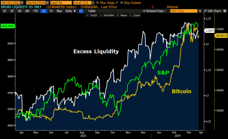Excess Liquidity, Bitcoin, and the S&PExcess liquidity have surged higher in the last year, which has pushed up risk assets, such as bitcoin and equities.

Together with the introduction of the BTFP in March ’23, the Fed and Treasury pushed up bank reserves from $3T on Oct 22, to $3.6T by March ’24. What do these reserves do? These reserves cannot leave the banking system and therefore cannot enter the “real economy”. It’s a financial form of money only for banks. They can transact in reserves with each other and settle repo and reverse repo transactions. They account for high-quality liquid assets (HQLA) together with bonds and mortgage-backed securities (MBS). Most importantly, banks use the reserves to buy bonds from each other. In this way, they drive liquidity into the market and drive investors into riskier assets. We see that almost every time reserves go up, risk assets benefit.

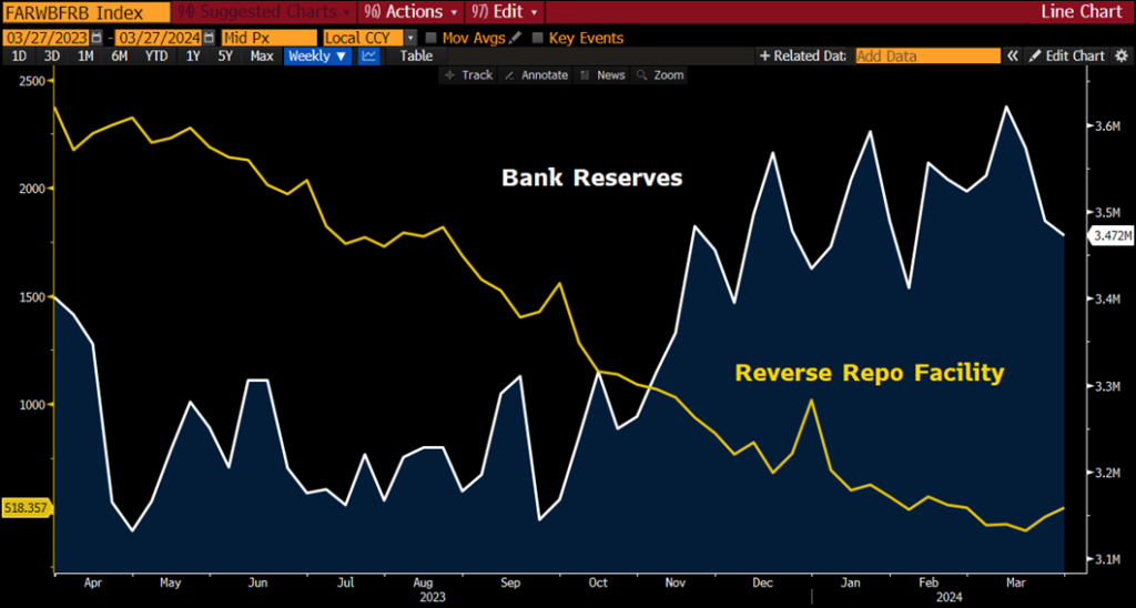Bank Reserves Go Up when RRP Goes Down and Vice VersaAs the Treasury pushed money out of the RRP, bank reserves held at the Fed have gone up simultaneously. This has been one of the biggest driver of stock market gains

In the next few weeks, we could see liquidity reverse for two reasons.

1) Treasury bill issuance will flip negative in Q2 to the tune of about $150bl. In Q1, 400bl of capital went from the RRP into the bills market, and in Q2 this will reverse. Add to that the 95bl in monthly QT and we could see 250bl of liquidity drain.

2) Expiration of the BTFP. In April about 75bl of BTFP loans expire and since the facility is now closed, they may not get renewed. This causes another contraction in bank reserves.

Overall we could see over $300bl of contraction if Yellen/Powell do not step in to offset. We think they will step in but it might take a month or so for them to react.

In the meantime, we are still in the buyback blackout window ($100bl of monthly buybacks do not start anew until after GOOG/AAPL report in late April/Early May) so we could fly into an air pocket.

In the next blog post, we will explain how Yellen and Powell can and will come up with a solution if they see liquidity plunge too far or stock market volatility surges higher.